Worked Example: Bead on a Ring

May 25, 2025

I recently worked through a problem that incorporated aspects of analytical mechanics and dynamical systems. Since it's such a great showcase of both techniques, I decided to share it here. The problem is simple:

Suppose you have a bead sliding along an upright ring, and the ring is rotating around a vertical axis at a constant speed. Describe the dynamics of the bead.

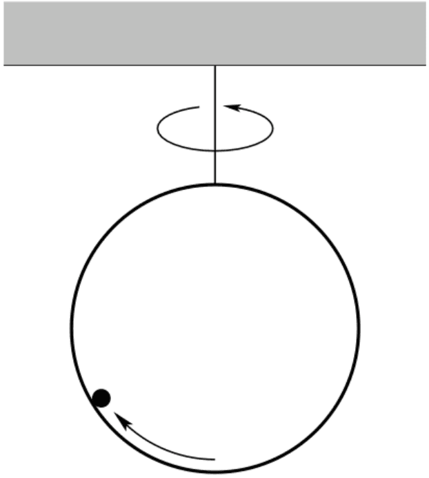
When the ring is still, we know the bead will simply rock back and forth. But as the ring begins spinning, we might expect that the centrifugal force causes the bead to be pushed towards the side. As it turns out, we can get a pretty precise answer to this problem!

The Equation of Motion

3Blue1Brown's advice for solving problems is that before anything else, we should give things names. So let's label the diagram from before.

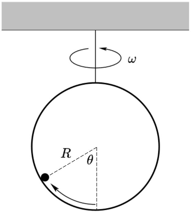
Here we have

• $\theta$ - the angle of the bead from the vertical
• $\omega$ - the rotating speed of the ring
• $R$ - the radius of the ring
• The bead has mass $m$ (not labeled)

We'll consider $R$ and $\omega$ as fixed (i.e. the ring rotates at a constant speed), so the only coordinate to vary is $\theta$. From here, we can use Lagrangian mechanics to determine how the system evolves.^[1] We end up getting

$$\ddot\theta = \tfrac12\omega^2\sin2\theta - \tfrac gR\sin\theta$$

The above equation, called the equation of motion for the system, tells us exactly how $\theta$ evolves over time. We can understand each term separately:

• Recall how $F = ma$, and acceleration is just the second derivative of position. This means that $\ddot\theta$ corresponds to the force applied to the bead, so the right-hand side tells us what the force is on the bead for each $\theta$.
• When $\omega = 0$, the first term vanishes and we're left with the equation of motion for a pendulum. This suggests that the $-\frac gR\sin\theta$ term accounts for gravity.
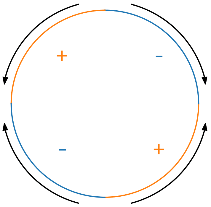
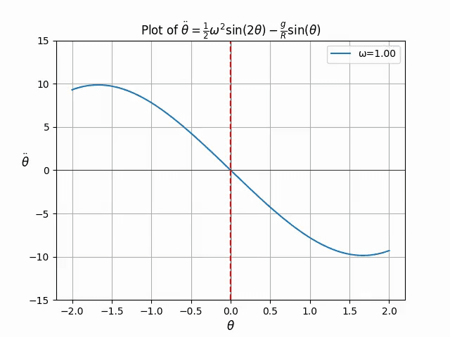
• The $\frac12\omega^2\sin2\theta$ term is responsible for the centrifugal force. The idea is that the $\sin2\theta$ pushes the bead towards the sides, changing sign depending on whether it's pushing clockwise or counterclockwise, while the $\frac12\omega^2$ controls the intensity. This sign-changing behavior is shown in the following image:

We can use the equation of motion to numerically simulate our system. Here are a few examples with $R = 1$ and $g = 9.81$. Note that because the equation of motion does not include $m$, it has no bearing on the dynamics of our system, so we don't need to specify it.

The centrifugal force gets stronger as $\omega$ grows. For smaller values of $\omega$, it simply slows the oscillation of the bead around the center. But as it grows larger, the bead is forced up against the sides of the ring. Looking at these videos, it seems like something happens between $3$ and $4$, since the bead stops oscillating around the center.

Dynamical Systems

It might seem that we've gone as far as we can go; nonlinear ODEs are hard to solve in general, and this one really seems hopeless. But there's quite a bit we can say without finding an explicit solution! The most noticeable thing is that center of oscillation changes with $\omega$: for small $\omega$, the bead oscillates around the center, but when $\omega$ passes a certain threshold, it starts oscillating around a higher point. How do these centers change? More generally, how can we describe the oscillations, stabilities and instabilities of our system?

The first step is to find the fixed points of our system, which occur when $\dot\theta = 0$ and $\ddot\theta = 0$, i.e. when the bead isn't moving and has no forces on it. The first condition is easy enough to understand: clearly the bead is not at a "fixed point" if it's moving. But the second one is a little harder. Since $\ddot\theta$ is a function of $\theta$, we need to find all $\theta$ such that $\ddot\theta = \frac12\omega^2\sin2\theta - \frac gR\sin\theta = 0$.

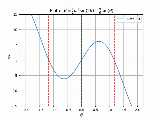
We can visualize the zeroes of $\ddot\theta$ by plotting the function directly. Fixing $R = 1$ and $g = 9.81$ as before, let's see what the zeroes are as we vary $\omega$.

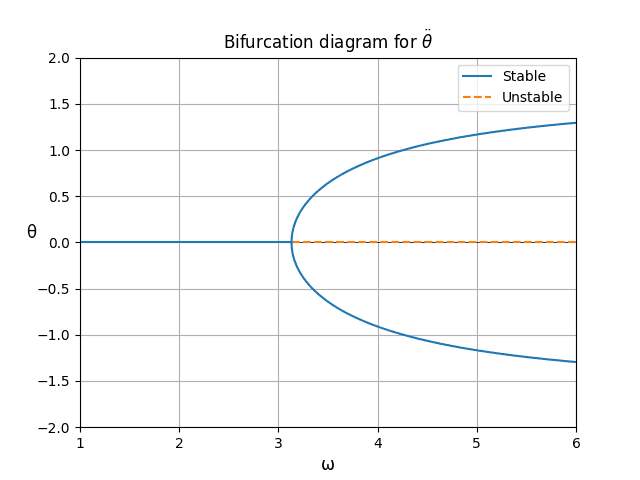
Interesting! It appears that as $\omega$ passes some threshold, we gain two new fixed points. This threshold turns out to be $|\omega| \geq \cos^{-1}(\frac{g}{R\omega^2})$.^[2] If we plot the locations of these fixed points versus the parameter $\omega$, we get

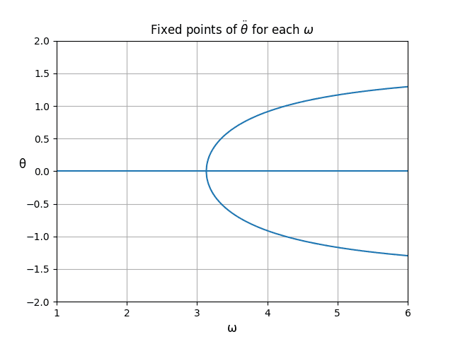
For small values of $\omega$, the only fixed point is in the center. But just past $\omega = 3$,^[3] the single fixed point splits into three. The above diagram is called a bifurcation diagram, and the specific form of this one is called a pitchfork bifurcation (you'll never guess why).

However, not all fixed points are created equal, which is why the next step is to discuss their stability. Stability can be perfectly encapsulated by the following image:

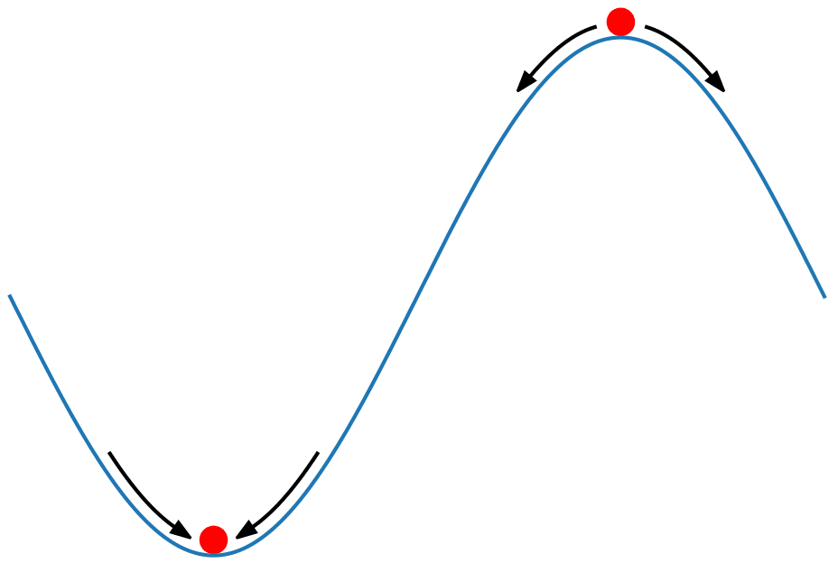
Consider two balls on a hill with the above configuration. Both are at fixed points, so under ideal conditions neither will move. But if we nudge each ball, the left one will return to the center while the right one will keep rolling away. We call the left fixed point stable and the right one unstable.

Returning back to our study of the bead on a ring, let's consider the stability of the fixed points of $\theta$. For the balls on the hill, we considered how the force of gravity behaved near the fixed points. We can do the same thing with the bead, recalling that $\ddot\theta$ represents the force on the bead. To that end, let's take a look at $\ddot\theta$ when $\omega = 1$.

When $\theta > 0$, $\ddot\theta$ is negative, pushing the bead back towards the center. Conversely, when $\theta < 0$, $\ddot\theta$ is positive, again pushing the bead back towards the center. It seems like the neighboring forces keep the bead at the origin, confirming that this fixed point is stable. We can compare this against the case when $\omega = 5$.

The two fixed points at $\theta = \pm1.17$ are stable for the same reason as above. However, the fixed point at $\theta = 0$ is no longer stable: for positive $\theta$, $\ddot\theta$ is also positive, pushing the bead further away from the center. The same thing happens for negative $\theta$, so we can say that this fixed point is unstable. We can amend our previous bifurcation diagram to reflect this shift in stability:

When the middle prong of a pitchfork is unstable while the rest is stable, we call it a supercritical pitchfork bifurcation. If you follow the diagram from right to left, you can think of the outer two fixed points coalescing into the center and absorbing the instability.

So the natural question to ask is, exactly when does the stable fixed point in the center become unstable? It turns out that this is very easy to answer. The transition happens when the slope of $\frac12\omega^2\sin2\theta - \frac gR\sin\theta$ at the origin turns from negative to positive, so we can just solve

$$\frac{\mathrm{d}}{\mathrm{d}\theta}(\tfrac12\omega^2\sin2\theta - \tfrac gR\sin\theta)\bigg|_{\theta=0} = 0$$

for $\omega$, which gives $|\omega| = \sqrt{\frac gR}$. So when the hoop is spinning slower than $\sqrt\frac gR$, the bead will always settle at the bottom, but not when it spins any faster.

Escaping the Cycle

The bead doesn't always have to oscillate around some point, though. We can imagine that if the bead started off spinning really quickly, it would just keep looping around the ring forever. The idea here is that at low speeds, the bead is stuck in an "energy valley" that's impossible to escape. But if the bead is going fast enough, it has the energy to escape the valley and summit the "energy hump", so to speak. We can illustrate this idea quite literally:

The top ball doesn't have enough energy to make it over the hill, so it stays stuck in the valley. But the bottom ball can make it over, so it keeps going forever.

Checking if the ball will make it over the hill is actually pretty easy: all we have to do is compute the energy of a still ball at the top of the hill. If our ball has that much energy, it'll make it over, and if it doesn't, then it'll remain stuck. The idea is that the summit is the highest energy state, so if the ball can make it over, then it has enough energy to reach any state.

It turns out that, because our system conserves energy, the highest-energy point is always an unstable fixed point. We already know about one unstable fixed point, the one at the bottom of the ring. But there's actually another you might not have noticed: the one at the top of the ring! This point has height $R$, so its potential energy is $mgh = mgR$. There's no kinetic energy since we're considering a still bead, so the total energy here is $mgR$.

The implication is that if a bead has energy at least $mgR$, then it'll make a full loop around the ring. For example, if we consider a bead starting at the bottom ($\theta = 0$), then its initial speed must be greater than $\dot\theta = 2\sqrt\frac gR$ to reach the top. We can see what happens when we're just above and just below this threshold:

A trajectory that divides the state space into isolated regions (in this case, "low-energy" and "high-energy") is called a separatrix, and the trajectory starting with $\dot\theta = 2\sqrt\frac gR$ is an example of one. As an aside, it's an interesting result that this initial speed does not depend on $\omega$ at all. Perhaps this is because the difficulty of rising to the top of the ring and resisting the centrifugal force is exactly counteracted by the boost that the centrifugal force gives when the bead first starts climbing.

1. I initially included a derivation of the equation of motion, but without a proper explanation of the method it seemed unmotivated. The steps are
   • Find the Lagrangian $\mathcal L = T - V$, the difference between kinetic and potential energy. For this system, we have $T = \frac12mR^2\dot\theta^2 + \frac12m\omega^2R^2\sin^2\theta$ and $V = -mgR\cos\theta$.
   • Substitute our expression for $\mathcal L$ into the Euler-Lagrange equation
   $$\frac{\mathrm{d}}{\mathrm{d}t}\frac{\partial\mathcal L}{\partial\dot\theta} - \frac{\partial\mathcal L}{\partial\theta} = 0$$
   • Solve the resulting equation for $\ddot\theta$
   It's a surprisingly easy set of steps, but delving into why this works is beyond the scope of this article, and it doesn't make sense to introduce it without an explanation. ↩
2. To see this, solve $\ddot\theta = 0$ for $\theta$ and leverage the identity $\sin2\theta = 2\sin\theta\cos\theta$. ↩
3. It actually splits at $\sqrt g \approx 3.13$, which is remarkably close to $\pi$. Surprisingly, this is not a coincidence, since hundreds of years ago, the meter was defined to satisfy the relation $\pi^2 = g$. More details here. ↩