What the **** is a Tensor?

September 6, 2023

A computer scientist will tell you that a tensor is a multidimensional array. Wikipedia says that a tensor is an "algebraic object describing a multilinear relationship". A physicist will just tell you that a tensor is anything that behaves like a tensor. Not helpful.

In this article we're going to explore a view of tensors that, to my knowledge, has not yet been presented on the internet. There's a big problem in linear algebra, and tensors are the unique objects that exactly solve this problem.

Almost Linear

Linear algebra is the study of linear functions, described above. It's unique in that, in a sense, the field is almost solved.^[1] If you've taken an intro course, you might have noticed that we have an extremely rich theory of how linear functions behave. So naturally, if we want to understand a function better, we might try to examine it from the perspective of linear algebra.

Consider the humble dot product, denoted by $\langle\cdot,\cdot\rangle$. If you've used it before, you'll know that it's kind of linear, but only in one argument at a time.

If it were linear, we would expect the $\lambda$ to distribute to all arguments.

But if you've used the dot product before, you know it doesn't work like that. This is a big problem, because it means all of linear algebra doesn't automatically apply. We can't talk about the null space, or eigenvalues, or anything like that. :(

Ideally, we'd like to "make" the dot product linear, which we can do by changing the space we're working in. Consider the map $M(u, v) = uv^\intercal$, which takes two vectors in $\mathbb R^3$ and gives us a matrix in $\mathbb R^{3 \times 3}$. More explicitly, it looks like

The dot product would then correspond to the sum of the diagonal entries, also known as the trace of a matrix. Except, you might notice something: the trace is linear! For any matrix $A$, we have

(Observe how the $\lambda$ distributes to all arguments). Somehow, we've turned a nonlinear function into a linear function, allowing us to employ the vast wealth of linear algebra knowledge we've accumulated over hundreds of years. To sum up the situation in a diagram,

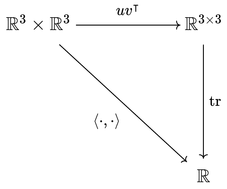
We can take the diagonal path directly using the dot product, or we can take a detour through $\mathbb R^{3 \times 3}$. If we take that detour, we get the bonus of having a linear function. Either way, you'll get the same answer.^[2] Take some time to really understand what this diagram is saying -- it's not obvious.

For any "almost linear" function (what we'd call bilinear), we can draw a similar diagram and get a linear function out of it.

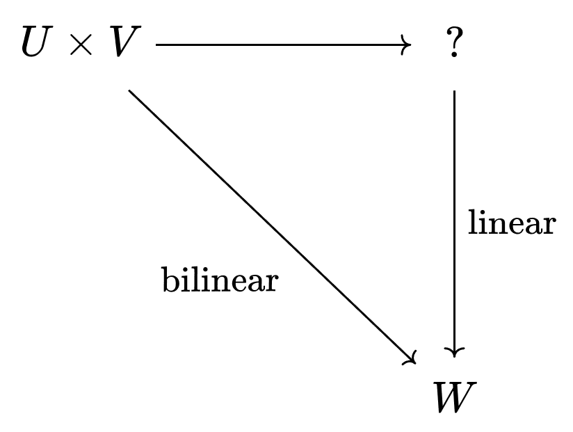
In our dot product example, we had $\mathbb R^{3 \times 3}$ in the top right. But in general, what should fill the spot of that question mark? Why, the tensor product of course!

The Tensor Product

The tensor product of two vector spaces, $U \otimes V$, lets us build a new, larger vector space that solves our linearity problem.^[3] Here's how it works:

1. For any two vectors $u, v$ in $U$ and $V$, we can "glue" them together using $\otimes$, and the resulting object, $u \otimes v$, is an element of $U \otimes V$. We call this object a tensor.
2. Pick bases $(u_i)$ and $(v_j)$ for $U$ and $V$. The basis for $U \otimes V$ then looks like every combination of $u_i \otimes v_j$.^[4] As a result, $\dim(U \otimes V) = \dim(U) \cdot \dim(V)$.
3. Scalars move freely around tensors. For any $u \otimes v$, we have $\lambda(u \otimes v) = \lambda u \otimes v = u \otimes \lambda v$. In other words, the magnitude of the tensor can be "shared" by its constituents.
4. Tensors are additive, so $(u + v) \otimes w = u \otimes w + v \otimes w$. The same is true for the other component as well.

Returning to our example, notice that $\dim(\mathbb R^3 \otimes \mathbb R^3) = \dim(\mathbb R^{3 \times 3}) = 9$ as we expect. More explicitly, the correspondence might look something like$$A_{ij} \Longleftrightarrow e_i \otimes e_j$$$$\begin{pmatrix} e_1 \otimes e_1 & e_1 \otimes e_2 & e_1 \otimes e_3 \\ e_2 \otimes e_1 & e_2 \otimes e_2 & e_2 \otimes e_3 \\ e_3 \otimes e_1 & e_3 \otimes e_2 & e_3 \otimes e_3 \end{pmatrix}$$ where $e_i$ is the standard basis for $\mathbb R^3$. Every matrix is the sum of 9 basis matrices, and every tensor is the sum of 9 basis tensors $e_i \otimes e_j$. But equipped with the general language of tensor products, we no longer need to talk about matrices to solve our linearity problem.

Note that not every tensor in $U \otimes V$ can be written as $u \otimes v$; in general, all tensors are the sum of simpler tensors, like $u_1 \otimes v_1 + \cdots + u_n \otimes v_n$. These simpler tensors are called pure tensors.

What Tensors Do for Us

Barring a couple details I omitted, what you see above is the full construction of the tensor product. What's so great about it? Going back to our problem from earler, remember that we wanted to turn a bilinear function into a linear one. The tensor product is the unique space that lets us do this. Finally, we can complete the diagram:

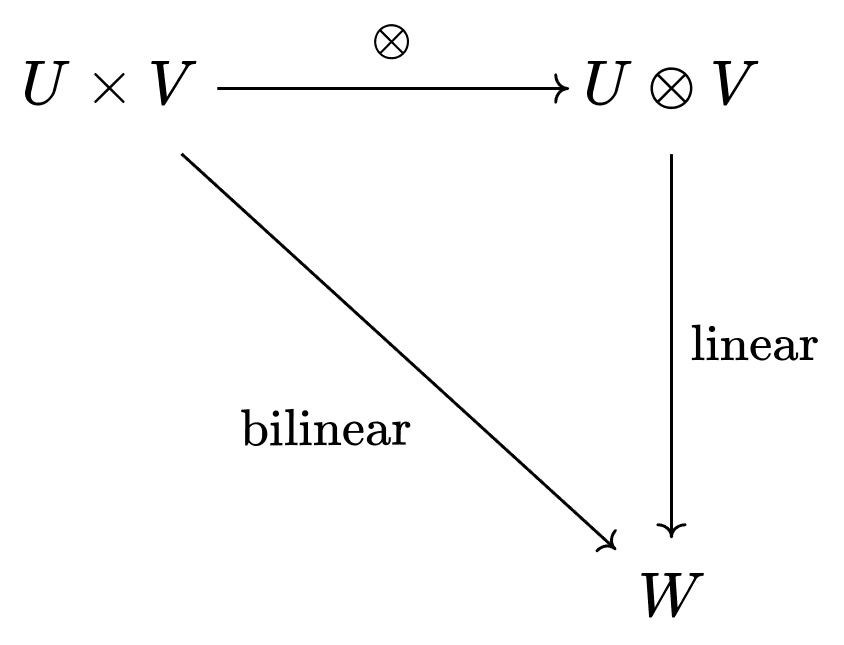
We wanted a linear map that agrees with the bilinear map on every input. $U \otimes V$ is the unique space that gives us a unique agreeing linear map.^[5] If we wanted, we could have a larger space containing $U \otimes V$, and we would certainly still have our linear map. But, it would no longer be unique.

The meaning of the $\otimes$ symbol may still be a little opaque, though; people will often ask "ok, but what is $u \otimes v$ really?  What's the $\otimes$ doing?"

Example: The Cauchy Stress Tensor

In essence, the job of the $\otimes$ is to emphasize the relationship between its constituent vectors. The fact that $\lambda u \otimes v = u \otimes \lambda v$ isn't just an algebraic rule; it tells us that we don't care where the $\lambda$ ends up. It doesn't belong to a vector, it belongs to the tensor.

This fact is well-illustrated by the Cauchy stress tensor. To model stress, we need two pieces of information: the force itself and the direction of the surface it acts on (this allows us to differentiate between shear vs. normal stress). However, we only want to keep track of one magnitude, the strength of the stress. Encoding these objects as tensors allows us to communicate that although there are two vectors present, we only care about their "shared" magnitude.

This is also why tensors are able to turn bilinear functions into linear ones. Bilinear functions allow the $\lambda$ to move around to any argument, and that's the defining property of tensors. As we said before, it doesn't matter where the $\lambda$ ends up; it doesn't belong to any individual argument, but to the tensor as a whole.

Addendum: Multilinearity

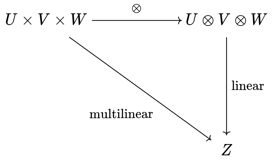
No discussion of tensors would be complete without the mention of multilinearity. Multilinearity is essentially the property of the dot product we discussed earlier, but extended to functions with any number of arguments. Specifically, we have that coefficients can jump between arguments,

and vectors in the same position can be added.

We can apply the tensor product to multilinear functions just as easily, allowing us to make any of them linear. We can even use the same diagram!

If you've taken an intro linear algebra course, you've already worked with a multilinear function: the determinant. Remember, if you scale any column of your matrix by $\lambda$, it scales the whole determinant by $\lambda$. It's no surprise that the determinant is used to model volume; multilinear functions are generally great at this, due to their scaling behavior and additivity.

1. This is a bit of an exaggeration, although there certainly is an element of truth to it. What's definitely true is that we have an extremely strong understanding of finite-dimensional linear algebra as presented in most introductory courses. Read this Math Stack Exchange answer for more context. ↩
2. A diagram like this, where you can take any path you want and get the same answer, is called a commutative diagram. They come from category theory, a language that attempts to describe mathematics in the most abstract terms possible -- it has been called "the mathematics of mathematics". ↩
3. Larger in the sense that $a \cdot b$ is typically larger than $a + b$. Recall that $\dim{A \times B} = \dim A + \dim B$. ↩
4. It's at this point that any mathematicians in the audience would complain that our construction is not basis-independent, to which I respond with two points:
   • The resulting space ends up being the same no matter which basis you choose.
   • The tensor product can be constructed using quotient spaces, as described in this article and in this excellent video by Michael Penn. Such a construction has the advantage of not requiring us to pick a basis, but it may be less intuitive. ↩
5. Unique up to a relabeling, of course. We could give each element of $U \otimes V$ a new name and it would still be the same thing. ↩